“Curve” is a term used liberally in general linguistic usage. From the scientific point of view a curve is a one-dimensional graph; that means simplified that the curve passes only in one direction - independent how smooth or spiky a curve pattern is. For example, raw data for glucose infusion rate (GIR) curves are notoriously spiky. This leads to a problem to calculate endpoints like GIRmax and tGIRmax because a single high peak / outlier may be identified as the maximum of the curve. Therefore these endpoints will be calculated from the smoothed curve instead of the raw curve.
At Profil , we generally use the mathematical procedure called LOESS (LOcal regrESSion) to smooth data. However, acceptable smoothing of data is a topic much debated and requires greater judgement than simply applying a mathematical formula. Hence, we thought we’d provide you with our thoughts on data smoothing.
What is the smoothing factor (SF)?
As you can imagine, Profil has analysed data from many thousands of glucose clamp experiments. The maximum GIR (GIRmax) and the time to achieve this (tGIRmax) are the key endpoints calculated. We use SAS® (SAS Institute Inc., Cary, North Carolina, USA) to perform LOESS, which – in statistical terms – is a non-parametric regression method to create smoothed data curves from the spiky raw data.
Delving deeper, LOESS enables application of either a linear or square mathematical function by using the weighted, least-squares method. LOESS is based on the Nearest-Neighbour-technique and requires input of what proportion of the surrounding values – known as the smoothing factor (SF) – at a particular time point will be used to calculate the smoothed value.
The SF is 1 or less. A SF of 1 would mean that all (100%) values surrounding a time point are included in the calculation to adjust that time point’s value to fit a smooth curve. When the SF is <1, then the calculation is limited to only those neighbouring data points within the represented proportion of data. For example, if SF=0.3, then 30% of the surrounding values will be used for calculation of a defined time point.
Why does the SF matter?
The SF is frequently debated, since different approaches to smooth the curve are available and data are transformed depending on the choice of SF. Some general points for consideration are:
- The higher the SF, the smoother and more generalized is the resultant curve
- The smaller the SF, the greater are the influence of the spikes of the raw data
Consider the following 3 examples each using the same range of 4 SFs:

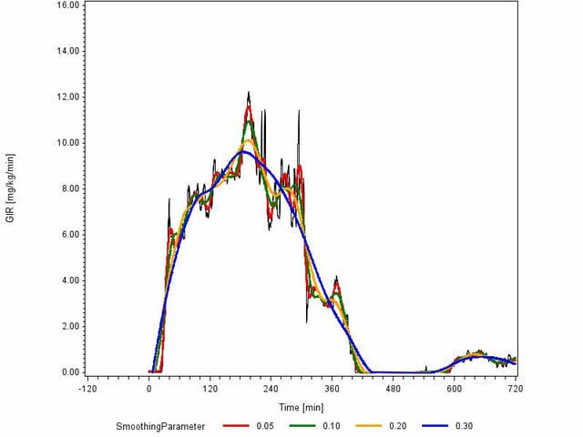
Example 1: For this short-acting insulin, resulting tGIRmax is close to being the same for all 4 SFs, but GIRmax itself differs considerably depending on the SF used. We can generalize here that the smaller the SF, the closer the GIRmax tends towards the raw data. Which SF is the more appropriate?

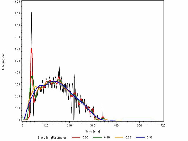
Example 2: For this second short-acting insulin, both tGIRmax and GIRmax differ depending on the SF used. The early outlier has a strong influence on the representation of the smaller SFs. Is that influence appropriate?

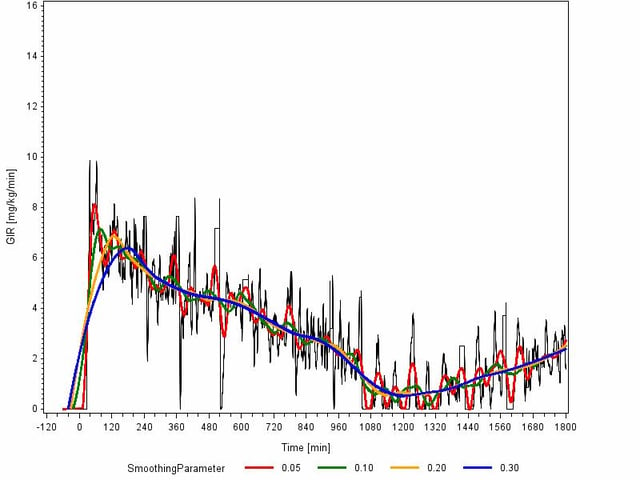
Example 3: For this long-acting insulin, both tGIRmax and GIRmax again differ depending on the SF used. The influences here would seem to be both the spiky nature of the raw data and potentially an early outlier. Which SF is the more appropriate here?
From these examples you will see that considerable distortion – intended or unintended – is possible from selection of SFs. Judgement on which SF is more appropriate in each case is far from simple and requires the balanced approach gained from experience.
Balancing interpretation of SF
On one side of the balance is the requirement not to impair your data by smoothing values too far from the actual data points measured (e.g., the SF is too large and tGirmax will be shifted (due to too strong smoothing) at a later time point as it is in reality). On the other side is the necessity to interpret complex data with a fair and reproducible analysis – and not with the aim to receive the most advantageous results.
Interpretation of SFs in publications warrant your critical consideration. Many publications present the SF without presentation of the criteria used for the selection or other quality criteria. The SFs may have been selected to show the most advantageous results. Presentation of multiple SFs for one profile can provide useful additional interpretive information when appropriate, though this requires careful management to avoid confusing reviewers with unwarranted nonsensical results.
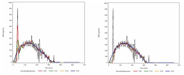
An alternative method is included in the LOESS procedure we use. SAS provides an iterative (repeated) reweighting method to improve the robustness of the smoothed curves in the presence of outliers – the effects of which are shown here:

Example 4: Comparison of LOESS without (left) and with (right) iterative reweighting.
From our experience gained over the years, we recommend using different SFs depending on whether the insulin being tested is short acting, long acting, or intermediate. The SF is usually in the range of 0.1 for short-acting insulin and around 0.25 for long-acting insulin.
Are your SFs being selected by experts?
Considering the influence SF selection can have a profound effect on interpretation of your data, we strongly recommend SF selection is done with appropriate care by an expert. Always trust your statistical analyses to statisticians who have experience in selecting and managing logical SFs for your particular field of study, such as are available in good full-service CROs like Profil . With our many years of experience in carrying out statistical analyses in diabetes trials, we have a dedicated team to take care of your analyses.


